ConfoundingWhat If: Chapter 7Elena Dudukina2021-02-041 / 14

Confounding

Lack of exchangeability

🧀

↙️ ↘️

🐿 🐿 🐿 🐿 🐿 🐿 🐿 🐿 🐿 🐿 🐿 🐿 🐿 🐿 🐿 🐿 🐿 🐿 🐿 🐿 🐿 🐿 🐿 🐿 🐿 🐿 🐿 🐿 🐿 🐿 🐿 🐿 🐿 🐿 🐿 🐿 🐿 🐿 🐿 🐿🐿 🐿 🐿 🐿 🐿 🐿 🐿 🐿 🐿 🐿 🐿 🐿 🐿 🐿 🐿 🐿 🐿 🐿 🐿 🐿 🐿 🐿 🐿 🐿 🐿 🐿 🐿 🐿 🐿 🐿 🐿 🐿 🐿 🐿 🐿 🐿 🐿 🐿 🐿 🐿 🐿 🐿 🐿 🐿 🐿 🐿 🐿 🐿 🐿 🐿 🐿 🐿 🐿 🐿🐿 🐿 🐿 🐿 🐿 🐿 🐿 🐿

🐭 🐭 🐭 🐭 🐭 🐭 🐭 🐭 🐭 🐭 🐭 🐭 🐭 🐭 🐭 🐭 🐭 🐭 🐭 🐭 🐭 🐭 🐭 🐭 🐭 🐭 🐭 🐭 🐭 🐭 🐭 🐭 🐭 🐭 🐭 🐭 🐭 🐭 🐭 🐭 🐭 🐭 🐭 🐭 🐭 🐭 🐭 🐭 🐭 🐭 🐭 🐭 🐭 🐭 🐭 🐭 🐭 🐭 🐭 🐭 🐭 🐭 🐭 🐭 🐭 🐭 🐭 🐭 🐭 🐭 🐭 🐭 🐭 🐭 🐭 🐭 🐭 🐭 🐭 🐭 🐭 🐭 🐭 🐭 🐭 🐭 🐭 🐭 🐭 🐭 🐭 🐭 🐭 🐭 🐭 🐭 🐭 🐭 🐭 🐭 🐭 🐭

2 / 14

7.1 The structure of confounding

Bias due to common causes

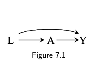
A: treatment
Y: outcome
L: confounder (a common cause of A and Y)

Paths between A and Y

A ➡️ Y: causal effect (directed path)
A ⬅️ L ➡️ Y: biasing backdoor path (starts with a head pointing into A)

The associational risk ratio $\frac{P r [Y = 1 | A = 1]}{P r [Y = 1 | A = 0]}$ is not causal risk ratio $\frac{P r [Y^{a} = 1]}{P r [Y^{a} = 0]}$

3 / 14

7.1 Examples

Occupational factors (healthy worker bias)

A: working as a firefighter
Y: mortality
L: being fit to work as a firefighter

Confounding by indication (channeling bias)

A: drug (aspirin)
Y: mortality
L: indication for the drug (heart disease)
U: (unmeasured) atherosclerosis

4 / 14

Lifestyle

A: behavior (exercise)
Y: mortality
L: lifestyle (smoking)
U: (unmeasured) personality/socioeconomic determinants

Reverse causation

A: behavior
Y: clinical disease
L: lifestyle (smoking)
U: (unmeasured) subclinical disease

5 / 14

Genetic factors (linkage disequilibrium)

A: DNA sequence
Y: developing a trait
L: DNA sequence confounding effect of A if L and A are often being inherited together and L causes Y
U: ethnicity

Social factors

A: income at age 65
Y: disability at age 75
L: disability at age 55
Time-varying flavor

Environmental exposures

A: airborne particle
Y: coronary heart disease
L: other pollutants, which levels co-vary together with A
U: (unmeasured) weather (controls the level of all types of airborne pollutants)

6 / 14

Assumptions for the remainder of the chapter

No selection bias (Chapter 8)
No measurement bias (Chapter 9)
No random variabiity (Chapter 10)

7 / 14

7.2 Confounding and exchangeabilityAssuming consistency and positivity holdExchangeability holds Ya⊥⊥A: potential outcome under the treatment regime is independent from actually observed treatment for all treatment levels (perfect randomization)
8 / 14

7.2 Confounding and exchangeability

Assuming consistency and positivity hold

Exchangeability holds $Y^{a} ⊥⊥ A$ : potential outcome under the treatment regime is independent from actually observed treatment for all treatment levels (perfect randomization)
When $Y^{a} ⊥⊥ A$ is true and treatment is binary
- the average causal effect $E [Y^{a = 1}] - E [Y^{a = 0}]$ equals the observed associational effect $E [Y | A = 1] - E [Y | A = 0]$

8 / 14

7.2 Confounding and exchangeability

Assuming consistency and positivity hold

Exchangeability holds $Y^{a} ⊥⊥ A$ : potential outcome under the treatment regime is independent from actually observed treatment for all treatment levels (perfect randomization)
When $Y^{a} ⊥⊥ A$ is true and treatment is binary
- the average causal effect $E [Y^{a = 1}] - E [Y^{a = 0}]$ equals the observed associational effect $E [Y | A = 1] - E [Y | A = 0]$
When conditional exchangeability holds $Y^{a} ⊥⊥ A | L$ , the verage caussal effect is identifiable
- $E [Y^{a = 1}] - E [Y^{a = 0}] = Σ_{l} E [Y | L = l, A = 1] * P r [L = l] - Σ_{l} E [Y | L = l, A = 0] * P r [L = l]$
- G-methods (IPTW, standardization) for marginal estimates

8 / 14

Is there a set of variables L that guarantees conditional exchangeability holds?No guarantees (unless well-conducted RCT)Use of DAGs to show the data-generating mechanism and assumptions
No residual confounding (conditional exchangeability) assumption
Backdoor criterion (J. Pearl, 1995)No node in adjustment set is a descendant (child) of exposure (not a mediator)
The adjustment set blocks all paths pointing into exposure (blocks all backdoor paths)
Consider magnitude and te direction of bias by unmeasured confounding

9 / 14

7.3 Confounding and the backdoor criterion

Adjustment sets sufficient to eliminate confounding:

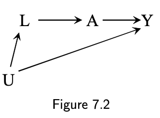
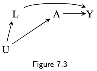
7.2: {L}, {U}

7.3: {L}, {U}
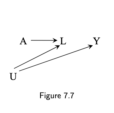
7.4: {} (empty set)
- adjusting for L opens a biasing path
- A ⬅️ U2 ➡️ [L] ⬅️ U1 ➡️ Y
think confounding, not confounders
role of the variable changes when other variables are adjusted

10 / 14

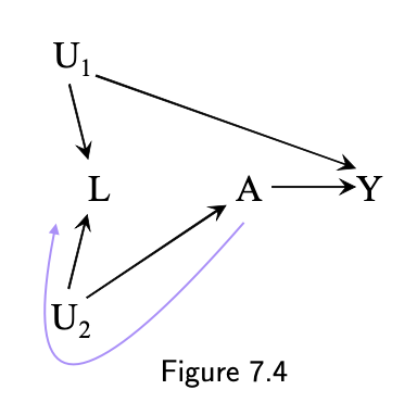
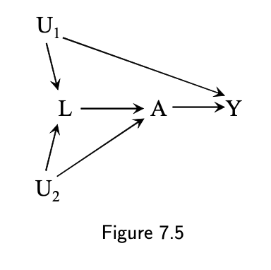
Fig 7.5

A ⬅️ L ⬅️ U1 ➡️ Y (open biasing path, L is not a collider)
A ⬅️ U2 ➡️ L ⬅️ U1 ➡️ Y (biasing path is closed with the collider L)
{U1}, {L, U2}, {L, U1}

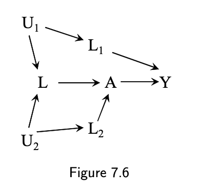
Fig 7.6

{L1}, {U1}, {L, L2}, {L, U2}, {L, L1}, {L, U1}

11 / 14

7.4 Confounding and confounders

Traditional criteria

Association with the exposure
Association with the outcome
Not on a causal pathway

Change of the estimate after adjustment may occur for the reasons other than adjusting confounding (selection bias, non-collapsibility of effect measures)

Is L a confounder?

12 / 14

7.6 Confounding adjustmentSufficient set for confounding adjustment
MethodsG-methods (marginal and conditional effects)Standardization
IP weighting (deleting an arrow L ➡️ A)
g-estimation

Stratification-based methods (conditional effects only)Stratification
Restriction
Matching


13 / 14

References

Hernán MA, Robins JM (2020). Causal Inference: What If. Boca Raton: Chapman & Hall/CRC (v. 31jan21)

14 / 14

Lack of exchangeability

🧀

↙️ ↘️

2 / 14

Help

Keyboard shortcuts

↑, ←, Pg Up, k

Go to previous slide

↓, →, Pg Dn, Space, j

Go to next slide

Home

Go to first slide

End

Go to last slide

Number + Return

Go to specific slide

b / m / f

Toggle blackout / mirrored / fullscreen mode

Clone slideshow

Toggle presenter mode

Restart the presentation timer

?, h

Toggle this help